Analog & Digital PID Controller Design

24 Oct 2023

INTRODUCTION

Proportional Integral Derivative (PID) controllers are the most used in the control industry. In this practice, different digital PID controllers will be simulated and tested using MATLAB SIMULINK. There are different methods used to design digital controllers but in this case, we will use one of them. The method consists in designing an analog PID controller and then using those parameters to recalculate digital PID parameters.

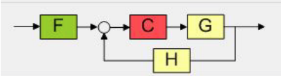
In the figure above, C is the controller, G is the transfer function of the system and H is the sensor transfer function or gain. Commonly, closed-loop control systems have. Three sample times will be used; thus, three different controllers for each method must be designed and tested. The sample times will be selected in order to obtain for the first method the following scenarios: a very similar performance, slight variations in performance and very different performance of the system with digital PID controller compared to the system with analog PID controller. Before starting to design digital PID controllers for a system, it is assumed that the transfer function of that system is known, and in the case of the first method, that the analog PID controller is also known. You should also know which are the design requirements for the controller.

THEORY

The following equation represents the analog PID in the time domain

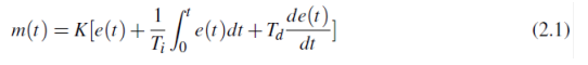
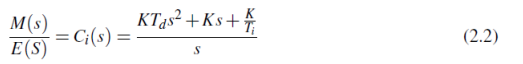
where e(t) is the error of the system and m(t) is the output of the analog PID controller. The Laplace representation of this controller results in the following transfer function:

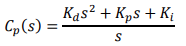
This representation is called the ideal PID Controller. Another form of the PID Controller is the parallel representation that has the following transfer function:

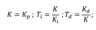
You can relate the parameters of these controllers from the following Equations:

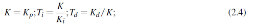
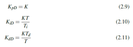
𝐾𝑝, 𝐾𝑖 and 𝐾𝑑 are the analog PID parameters in the parallel form and K, 𝑇𝑖 and 𝑇𝑑 are the analog PID parameters in the ideal form. The approximations used to obtain the discrete representation of the analog PID controller are

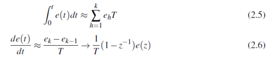
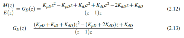
where T is the sampling time. Then, the digital PID controller has the following equation:

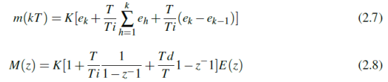
Then, the digital PID controller has the following transfer function:

PID controllers, which are usually recognized as the most often used controllers in the control sector, play a crucial role in the field of control systems. Using the mathematical formulas and powerful Matlab Simulink program, we examine the theory, the simulation and testing of analog and various digital PID controllers in this research. Different approaches can be used while designing analog and digital controllers, however for the sake of this study, we’ll concentrate on one particular methodology. In our approach, an analog PID controller is first designed, and the digital PID controller is then calibrated using the obtained parameters. We can bridge the gap between analog and digital control systems by utilizing this method.

AIMS AND OBJECTIVES

This study’s main goal is to investigate how to create digital PID controllers from analog controllers that are already available and compare digital with different sampling times and digital with analog controllers. We have determined the following precise goals with this end in mind:

For the Speed Control System, digital PID controller design: The main focus will be on developing digital PID controllers specifically suited for the Speed Control System using the techniques described in the documentation provided. The goal is to complete all of the system’s design specifications.

In order to evaluate how well digital PID controllers operate at various sampling rates: We try to find out how changing the sampling times affects how well digital PID controllers work. By comparing the two, we hope to learn more about the advantages and drawbacks of the various sampling times as well as how they affect the performance of the system as a whole.

The Speed Control System’s digital PID controllers will be put through testing and verification as follows: After being designed, it is crucial to put the digital PID controllers through a test in the speed control system. In order to determine whether the system’s design requirements have been successfully met, it is important to assess each controller’s performance.

By achieving these aims and objectives, we aim to advance our knowledge and understanding of digital and analog PID controller design, performance evaluation, and verification processes. The outcomes of this study will facilitate the development of optimized control strategies and contribute to enhancing the efficiency and effectiveness of control systems, particularly in the context of the Speed Control System

RESULTS & DISCUSSIONS

Speed Control System Parallel PID Controller Representation:

• 𝐾𝑝, 𝐾𝑖 ,𝐾𝑑 𝑎𝑟𝑒 𝑡ℎ𝑒 𝑎𝑛𝑎𝑙𝑜𝑔 𝑃𝐼𝐷 𝑝𝑎𝑟𝑎𝑚𝑒𝑡𝑒𝑟𝑠 𝑖𝑛 𝑡ℎ𝑒 𝒑𝒂𝒓𝒂𝒍𝒍𝒆𝒍 𝒇𝒐𝒓𝒎 𝒂𝒏𝒅 𝐾, 𝑇𝑖 , 𝑇𝑑 𝑎𝑟𝑒 𝑎𝑛𝑎𝑙𝑜𝑔 𝑃𝐼𝐷 𝑝𝑎𝑟𝑎𝑚𝑒𝑡𝑒𝑟𝑠 𝑖𝑛 𝑡ℎ𝑒 𝒊𝒅𝒆𝒂𝒍 𝒇𝒐𝒓𝒎

Analog PID Controller

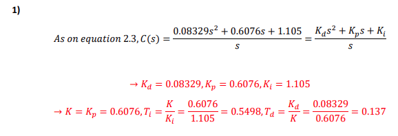
1) Let’s obtain the Analog PID parameters from the analog PID Controller by using 2.3 & 2.4

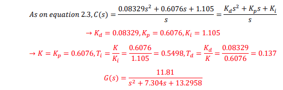
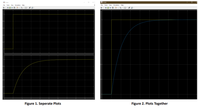
2) We simulate the Analog PID Controller and plot the system output.

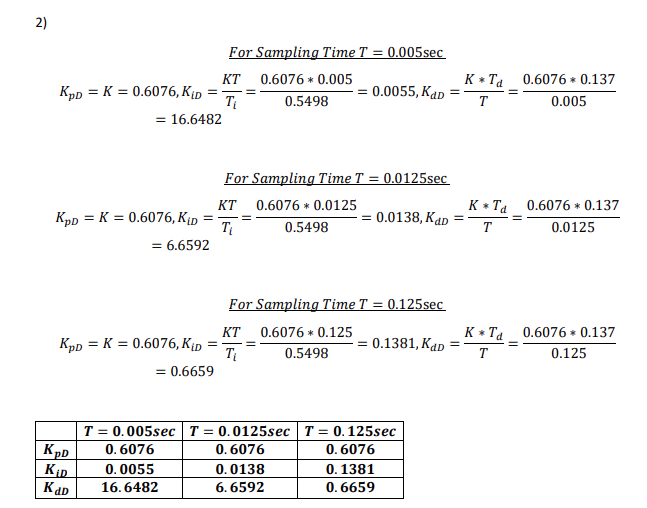
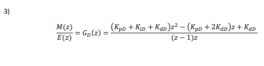
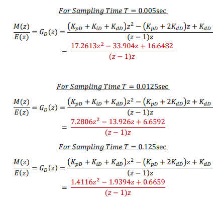
Digital PID Controller

COMMENT

Analog System

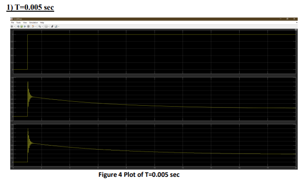
Overshoot means or refers to how far we go over the desired or reference value. Overshoot of the system is almost 0 percent as we can see from the graph and this means that we don’t have that much instability. The settling time is almost equal to the rising time which means the system is reaching its steady state value very quickly without significant overshoot or oscillation. Steady state error is lower as well, the steady state error is the difference between the desired output, setpoint and the actual output of the system once it has reached steady state, a low steady state error means that system is accurately reaching the desired output, so we can say that the system is steady. Furthermore, let’s talk about the control parameters which are 𝑲𝒑, 𝑲𝒅, 𝑲𝒊 . Proportional constant determines how aggressively the system responds to an error. A higher value will make the system respond more quickly, but can also lead to more overshoot and instability. Derivative constant helps to predict the system’s future behavior and can reduce overshoot and improve stability. On the other hand, it can also make the system more sensitive to noise. Integral constant helps to eliminate steady state error, but can also lead to overshoot and longer settling times if it’s too large

Digital System

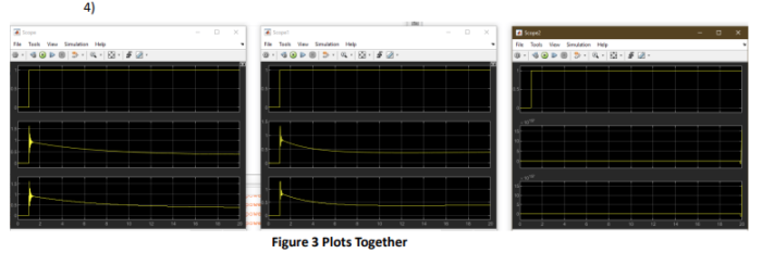
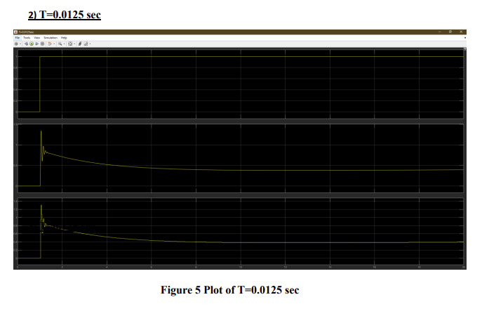
As the sample time increases, the oscillation in the system decreases, but the steady state error increases. Especially in the last system, sampling time is very high, but control is almost non-existent it is problem. Steady state error is very high, and we have oscillation, so it is not a very stable system. As the sample time increases, the derivative decreases, so the oscillation decreases, but after a point there is no control which causes problem, so we need to be careful while selecting the numbers. It can be said that it is more unstable than the analog PID controller. From the graphs we can see that overshoot is decreasing with the increase of sampling time. Settling time seems to be decreasing as the sampling time increases until some point after that the control is not well so we can’t clearly analyze that part (e.g. T=0.125sec). Rising time increases as the sampling time increases and again after some time the system is not working well. Steady-state error increases as the sampling time increases. Analog controllers have less steady state error, provide smoother, continuous control, potentially leading to less overshoot and faster settling and rise times. Digital controllers offer precise control, while their performance can be affected by the sampling rate.

CONCLUSION

In summary, in this project we examined the design, simulation, and testing of digital PID controllers for the Speed Control System. The project involved the design of digital controllers from pre-existing analog controllers and compares their performance under different sampling times. The aim was to meet design specifications and assess performance. The efficiency of the designed controllers in meeting the system’s performance expectations has been achieved. This was achieved by utilizing the methodology outlined in this project, resulting in the successful design of digital PID controllers for the Speed Control System. Leveraging the parameters that were derived from the analog PID controllers allowed for the effective translation of analog control strategies. Converted into digital counterparts. This approach allowed us to bridge the difference between analogue and digital control systems and ensured a seamless transition from theory to practical application.

REFERENCES

[1] Basic introduction to feedback control, https://www.eecs.umich.edu/courses/eecs373.w05/lecture/control.html (accessed Jun. 15, 2023).